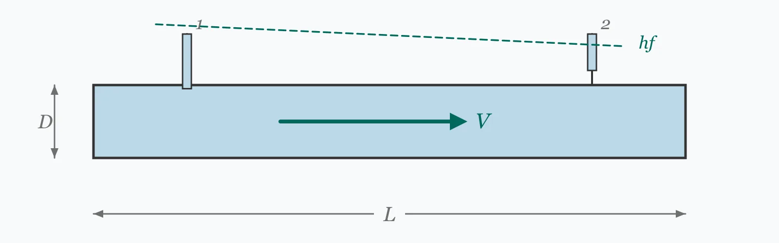
Friction head loss follows Darcy-Weisbach: hf = f·(L/D)·(V²/2g). Enter the friction factor, pipe length, diameter and velocity to get the head loss, the equivalent pressure drop and the pumping power it consumes. The power figure is what makes pipe sizing an energy decision rather than a material one.
Calculator
Units:
—
0.015–0.03 typical for water in commercial pipe; 64/Re if laminar
m
Straight pipe length; add equivalent lengths for fittings
mm
Internal bore diameter
m/s
Mean flow velocity in the pipe
Calculation Result
Press Calculate for the head loss in metres, the pressure drop in kPa, the loss per metre of pipe, and the power required to overcome it. The power figure is the annual energy cost in disguise.
Step-by-Step Solution
Preliminary design aid. Results follow the published formulas cited
below and are intended for estimating, study and early design. Final design must be
verified by a licensed Professional Engineer against the code in force for your project.
Key Benefits
✓Applies the Darcy-Weisbach equation, valid for any fluid and any flow regime
✓Converts head loss into both pressure drop and pumping power
✓Reports loss per metre, the figure used for comparing pipe runs
✓Includes friction factor guidance and the Moody chart context
✓Sensitivity chart shows the quadratic dependence on velocity
✓Shareable links and CSV export for hydraulic calculations
What Is Head Loss?
As fluid moves through a pipe, friction against the wall and internal shear convert mechanical energy into heat. Darcy-Weisbach expresses that loss as a head — a height of fluid column — through hf = f·(L/D)·(V²/2g). The velocity head V²/2g is the kinetic energy per unit weight, and the factor f·L/D scales it by how much pipe the fluid has passed through relative to its diameter.
Where the friction factor comes from
The friction factor f is the empirical part. In laminar flow it is exactly 64/Re. In turbulent flow it depends on both the Reynolds number and the relative roughness ε/D, through the implicit Colebrook equation, or graphically through the Moody chart. For water in commercial pipes at ordinary velocities, f typically lands between 0.015 and 0.03, and 0.02 is a reasonable first estimate.
Why diameter dominates the energy cost
At a fixed flow rate, velocity is inversely proportional to D², so V² goes as 1/D⁴, and dividing by D in the equation gives head loss proportional to 1/D⁵. Increasing a 100 mm pipe to 150 mm — one and a half times the diameter — cuts friction loss by a factor of about 7.6. That is why pipe sizing on capital cost alone systematically undersizes: the energy consumed over the life of the system usually dwarfs the difference in pipe cost.
Formula
h_f = f · (L/D) · (V² / 2g)
Darcy-Weisbach friction head loss in a pipe
Related Formulas
ΔP = ρ g h_f
P = γ Q h_f
f = 64 / Re
1/√f = −2 log₁₀(ε/3.7D + 2.51/(Re√f))
Variable Definitions
Symbol
Variable
Unit
Description
h_f
Head Loss
m
Energy lost to friction, expressed as a height of the flowing fluid.
f
Friction Factor
—
Darcy friction factor. 0.015 to 0.03 for water in commercial pipes; exactly 64/Re if laminar.
L
Pipe Length
m
Length of pipe over which the loss accumulates. Head loss is directly proportional to it.
D
Pipe Diameter
mm
Internal bore. At fixed flow, head loss varies as the inverse fifth power of this.
V
Flow Velocity
m/s
Mean velocity. Head loss goes with its square.
ΔP
Pressure Drop
kPa
Head loss converted to pressure through ρg.
How to Use This Calculator
Choose the friction factor from the regime and roughnessFor laminar flow, f = 64/Re exactly. For turbulent flow, use a Moody chart or the Colebrook equation with the relative roughness ε/D. Commercial steel has ε ≈ 0.045 mm, plastic ≈ 0.0015 mm, and old cast iron can exceed 1 mm.
Include fittings as equivalent lengthBends, valves and fittings add local losses, usually handled by converting each to an equivalent length of straight pipe. A gate valve is around 8 diameters, a standard elbow 30, and a globe valve can exceed 300.
Use the internal bore, not the nominal sizeHead loss varies as 1/D at fixed velocity and 1/D⁵ at fixed flow, so bore accuracy matters more here than almost anywhere else. Allow for lining thickness on lined pipe.
Read the power loss as an annual costThe power figure is continuous hydraulic power. Divide by the pump efficiency, multiply by annual running hours and by the electricity tariff to get the operating cost — which is what justifies a larger pipe.
Add the static lift for the pump dutyFriction loss is only part of the pump head. The total duty is the static lift plus all friction and fitting losses, and the pump is selected against that total at the design flow.
Worked Examples
Example 1
Water flows at 1.5 m/s through 100 m of 150 mm pipe with a friction factor of 0.02. Find the head loss, pressure drop and pumping power.
Head loss: hf = f × (L/D) × (V²/2g) = 0.02 × 666.7 × 0.11468
hf = 1.529 m
Pressure drop: ΔP = 9.81 × 1.529 = 15.00 kPa
Head loss per metre: 1.529 / 100 = 0.01529 m/m
Flow rate: Q = V × A = 1.5 × π × 0.15²/4 = 0.026507 m³/s
Power: P = γQhf = 9,810 × 0.026507 × 1.529 = 397.6 W
Example 2
The same 26.5 L/s flow through 100 mm pipe instead of 150 mm. This is the calculation that decides pipe size on any pumped system.
Step-by-Step Solution
Velocity in the 100 mm pipe: V = Q/A = 0.026507 / (π × 0.1²/4) = 3.375 m/s
Velocity head: 3.375² / 19.62 = 0.5806 m
L/D = 100 / 0.1 = 1,000
Head loss: hf = 0.02 × 1,000 × 0.5806 = 11.611 m
Pressure drop: 9.81 × 11.611 = 113.91 kPa
Power: 9,810 × 0.026507 × 11.611 = 3,019.3 W
Comparison against the 150 mm pipe: head loss rose from 1.529 to 11.611 m, and power from 398 W to 3,019 W — a factor of 7.6
The scaling is (150/100)⁵ = 7.59, exactly matching. Head loss at constant flow varies as the inverse fifth power of diameter.
The economics: 2.6 kW of extra pumping power running continuously is roughly 23,000 kWh a year. At any realistic tariff that dwarfs the cost difference between 100 mm and 150 mm pipe within the first year or two.
Velocity Sensitivity
Head loss rises with the square of velocity, and power with its cube — because power is head loss times flow rate, and both are rising. Switch to the power curve to see how steeply the energy cost climbs. The marker shows your current velocity.
Head Loss (hf) vs Flow Velocity (V)
Recomputed live from your inputs. The marker shows your current value.
Line chart of Head Loss (hf) against Flow Velocity (V). The same
values are listed in the data table below.
Values plotted above, sampled across the flow velocity (v) range.
How to Interpret Your Results
Head loss per metre is the figure to compare between options, since it is independent of the run length. The power output is the one that turns a hydraulic result into an economic argument.
Head Loss per Meter: < 0.005Low friction gradient
A gradient of your result m/m is low, indicating a generously sized pipe. Pumping cost will be modest, though check that the resulting velocity is still above the self-cleansing minimum if the fluid carries solids.
Head Loss per Meter: 0.005 – 0.03Normal design range
A gradient of your result m/m is the range most pumped systems are designed to. It balances pipe capital cost against pumping energy over the life of the installation.
Head Loss per Meter: 0.03 – 0.1High friction gradient
A gradient of your result m/m is steep. Over a long run this becomes the dominant part of the pump duty. Because head loss varies as the inverse fifth power of diameter at constant flow, one pipe size up will cut it dramatically.
Head Loss per Meter: ≥ 0.1Excessive friction gradient
A gradient of your result m/m is very high and suggests a substantially undersized pipe. Verify the velocity against the erosion limit as well — high friction gradients and excessive velocity almost always occur together.
Power Required: ≥ 1000Significant pumping power
A friction power of your result W is a continuous energy cost. Divide by the pump efficiency and multiply by annual running hours: at 1 kW running continuously, that is roughly 8,760 kWh a year before pump losses. Compare against the cost of a larger pipe.
Common Mistakes to Avoid
Using a fixed friction factor regardless of regime
Why it matters:In laminar flow f = 64/Re and can exceed 0.1, far above the 0.02 typical of turbulent water flow. Applying a turbulent value to laminar flow understates the loss by several times.
✓How to avoid it:Check the Reynolds number first. Use 64/Re below 2,300, and a Moody chart or the Colebrook equation above 4,000.
Ignoring fittings and valves
Why it matters:Local losses at bends, valves and changes of section can exceed the straight pipe friction in a compact installation. A single globe valve is worth over 300 pipe diameters of straight run.
✓How to avoid it:Convert each fitting to an equivalent length and add it to the pipe length, or use K-factors and add the local losses separately.
Sizing pipes on capital cost alone
Why it matters:Head loss varies as the inverse fifth power of diameter at constant flow, so a slightly larger pipe cuts pumping energy dramatically. On a continuously running system, the energy saving typically repays the pipe cost within a year or two.
✓How to avoid it:Compare total lifetime cost — pipe plus pumping energy — rather than pipe cost alone. This is a standard economic pipe diameter calculation.
Using nominal diameter instead of internal bore
Why it matters:Because head loss varies so steeply with diameter, a small bore error produces a large error in the result. A 5% bore reduction raises head loss by about 28% at constant flow.
✓How to avoid it:Take the internal diameter from the pipe schedule, allowing for any lining. This matters more in head loss calculations than in almost any other hydraulic check.
Forgetting the static lift in the pump duty
Why it matters:Friction loss is only one component of pump head. A pump selected on friction alone will not deliver against the elevation the system also has to overcome.
✓How to avoid it:Total pump head is static lift plus friction plus fitting losses, evaluated at the design flow. Plot the system curve against the pump curve to find the true operating point.
Applying Hazen-Williams outside its range
Why it matters:Hazen-Williams is a convenient alternative but is empirical, calibrated for water at ordinary temperatures and velocities. It has no viscosity term and becomes unreliable for other fluids or unusual conditions.
✓How to avoid it:Use Darcy-Weisbach where the fluid is not cold water, where the flow may be laminar, or where accuracy matters. Hazen-Williams is a shortcut, not an equivalent.
Practical Applications
▸Sizing pumps for water distribution and circulation systems
▸Comparing pipe diameter options on lifetime cost
▸Calculating pressure available at the far end of a run
▸Assessing existing systems under increased flow demand
▸Determining pumping energy cost for operating budgets
▸Checking pressure drop in process and cooling circuits
Industry Use Cases
Water distribution
Long transmission mains are sized by economic optimisation rather than by velocity limits alone. The calculation weighs pipe capital cost against the discounted pumping energy over the design life, and the optimum usually sits at a lower velocity than a purely hydraulic view would choose.
Building services
Heating and chilled water circuits are designed to a friction gradient rather than a velocity, commonly around 100 to 300 Pa/m. Working to a gradient keeps the whole network balanced and makes the pump duty predictable.
Process and mining slurry
Slurry pipelines must stay above a critical deposition velocity to keep solids suspended, but friction rises steeply with velocity. The design window between settling and excessive wear is narrow, and head loss calculations sit at the centre of it.
Expert Tips
💡At constant flow, head loss varies as the inverse fifth power of diameter — one size up is transformative.
💡Power goes as the cube of velocity, so a 20% velocity reduction cuts pumping power by 42%.
💡Design to a friction gradient rather than a velocity where a whole network must balance.
💡Fittings can dominate in compact installations — a globe valve is worth 300 diameters of pipe.
💡For water, pressure drop in kPa is simply 9.81 times the head loss in metres.
💡Check the Reynolds number before picking a friction factor; laminar and turbulent values differ severalfold.
Advantages & Limitations
Advantages
✓Darcy-Weisbach is dimensionally consistent and valid for any fluid and regime
✓Returns pressure drop and pumping power alongside the head loss
✓Loss per metre allows direct comparison between pipe options
✓Extends to fittings through equivalent lengths
✓Fast enough to compare diameters during design
Limitations
!Requires the friction factor as an input rather than deriving it from roughness and Reynolds number
!Covers straight pipe friction only; fittings must be added as equivalent length
!Assumes a full, circular, pressurised pipe of constant section
!Assumes steady flow — surge and water hammer are separate calculations
!The pressure drop conversion assumes water density; other fluids need scaling by relative density
!Takes no account of pipe ageing, which increases roughness substantially over decades
!Does not compute the system curve or the pump operating point
Head Loss by Diameter at Constant Flow
The same 26.5 L/s through 100 m of pipe at f = 0.02. The fifth-power relationship is what makes pipe sizing an energy decision: the power column falls a hundredfold across this range.
Water at 26.5 L/s through 100 m of pipe, f = 0.02 throughout. In reality f varies somewhat with diameter and Reynolds number.
Use Darcy-Weisbach: hf = f·(L/D)·(V²/2g). For water at 1.5 m/s through 100 m of 150 mm pipe with f = 0.02, that gives 1.529 m of head, equivalent to 15.0 kPa.
What is the Darcy friction factor?
A dimensionless coefficient capturing wall friction. In laminar flow it is exactly 64/Re. In turbulent flow it depends on Reynolds number and relative roughness through the Colebrook equation, and typically lands between 0.015 and 0.03 for water in commercial pipe.
How does pipe diameter affect head loss?
Dramatically. At constant flow rate, head loss varies as the inverse fifth power of diameter. Going from 100 mm to 150 mm cuts it by a factor of 7.6, which is usually enough to repay the extra pipe cost in energy within a year or two.
How do I convert head loss to pressure drop?
Multiply by ρg. For water, pressure drop in kPa is simply 9.81 times the head loss in metres. So 1.529 m of head is 15.0 kPa. For other fluids, scale by relative density.
How much pumping power does friction cost?
P = γQhf, giving hydraulic power in watts with γ = 9,810 N/m³ for water. Divide by pump efficiency for shaft power, and by motor efficiency again for electrical input.
Should I use Darcy-Weisbach or Hazen-Williams?
Darcy-Weisbach is fundamental and applies to any fluid and any regime. Hazen-Williams is an empirical shortcut calibrated for cold water at ordinary velocities, with no viscosity term, so it becomes unreliable outside those conditions.
How do I account for bends and valves?
Convert each to an equivalent length of straight pipe and add it to L. A gate valve is around 8 diameters, a standard elbow 30, and a globe valve over 300 — which is why valve selection matters as much as pipe sizing in compact plant.
What is a typical friction gradient for design?
Building services circuits commonly work to 100 to 300 Pa/m, roughly 0.01 to 0.03 m/m. Long transmission mains are sized by economic optimisation instead, and often land at a lower gradient because the energy cost dominates.
Does pipe roughness change over time?
Substantially. Corrosion, scaling and biofilm all increase roughness, and an old cast iron main can have several times its original friction factor. Design for the aged condition, not the new-pipe value, on any long-life system.
Why does pumping power rise so steeply with velocity?
Because power is head loss times flow rate, and both rise with velocity. Head loss goes as V² and flow as V, so power goes as V³. A 20% velocity reduction cuts pumping power by 42%.
Glossary
Head loss
Energy lost to friction, expressed as an equivalent height of the flowing fluid.
Darcy-Weisbach equation
The fundamental relationship hf = f(L/D)(V²/2g) for friction loss in a pipe.
Friction factor (f)
A dimensionless coefficient depending on Reynolds number and relative roughness.
Velocity head
The quantity V²/2g, representing kinetic energy per unit weight of fluid.
Relative roughness
Wall roughness height divided by pipe diameter, ε/D, the parameter governing turbulent friction.
Moody chart
A graphical solution of the friction factor against Reynolds number for a family of relative roughnesses.
Equivalent length
The length of straight pipe producing the same loss as a given fitting or valve.
Friction gradient
Head loss per unit length of pipe, used to compare and balance networks.
System curve
The relationship between flow and required head for a system, whose intersection with the pump curve sets the operating point.
Scientific & Standards References
Moody, L. F., Friction Factors for Pipe Flow, Transactions ASME 66 (1944) — American Society of Mechanical Engineers
Colebrook, C. F., Turbulent Flow in Pipes, Journal of the ICE (1939) — Institution of Civil Engineers
Crane Technical Paper No. 410 — Flow of Fluids Through Valves, Fittings and Pipe — Crane Co.
White, F. M., Fluid Mechanics, 8th Edition — Chapter 6: Viscous Flow in Ducts — McGraw-Hill
CIBSE Guide C — Reference Data: Flow of Fluids in Pipes and Ducts — Chartered Institution of Building Services Engineers
Conclusion
Darcy-Weisbach gives friction head loss as f·(L/D)·(V²/2g), and its exponents are what matter in practice. Head loss goes with the square of velocity and inversely with diameter, which at fixed flow rate combines into an inverse fifth power of diameter — so one pipe size up cuts friction by a factor of seven or more. Pumping power goes further still, as the cube of velocity. Together these make pipe sizing an economic optimisation rather than a hydraulic one: on any continuously running system, the energy saved by a larger pipe typically repays its capital cost within a year or two. The friction factor is the input worth care, since laminar and turbulent values differ severalfold and old pipe is rougher than new.
Check your own run above, then sweep the velocity in the chart to see how steeply the pumping power climbs.