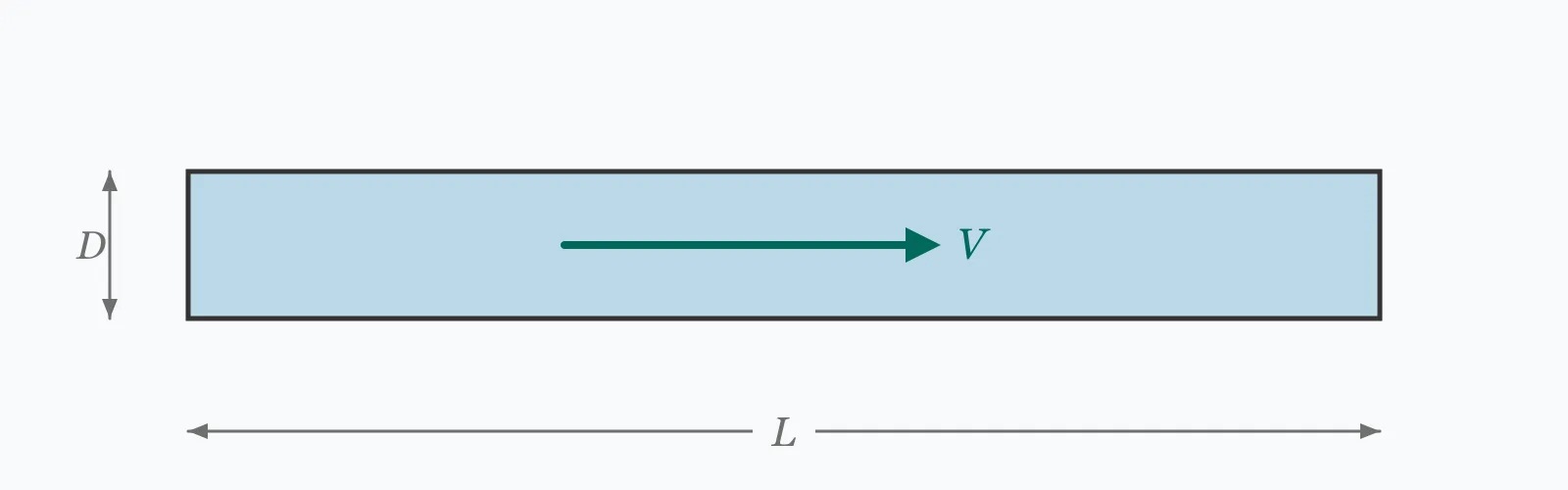
Velocity in a full pipe is simply flow rate divided by area, V = Q/A. The Reynolds number Re = VD/ν then tells you whether that flow is laminar, transitional or turbulent — which decides everything downstream, from friction factor to mixing behaviour. Enter flow rate, diameter and kinematic viscosity to get all four.
Calculator
Units:
L/s
Volumetric flow through the pipe
mm
Internal bore diameter, not the nominal size
×10⁻⁶ m²/s
Water at 20 °C = 1.004; at 5 °C = 1.52; at 60 °C = 0.47
Calculation Result
Press Calculate for the flow velocity, Reynolds number, flow regime code and pipe area. The regime code is 1 for laminar, 2 for transitional and 3 for turbulent.
Step-by-Step Solution
Preliminary design aid. Results follow the published formulas cited
below and are intended for estimating, study and early design. Final design must be
verified by a licensed Professional Engineer against the code in force for your project.
Key Benefits
✓Returns velocity, Reynolds number and flow regime in one pass
✓Classifies the regime explicitly rather than leaving the reader to interpret Re
✓Warns automatically when velocity exceeds the 3 m/s erosion threshold
✓Includes the design velocity ranges used for water, drainage and process pipework
✓Sensitivity chart shows how sharply velocity falls with diameter
✓Shareable links and CSV export for design records
What Is Pipe Flow?
For a pipe running full, continuity gives the mean velocity directly: Q = VA, so V = Q/A with A = πD²/4. Because area goes as the square of diameter, velocity is inversely proportional to D². Doubling the pipe diameter at constant flow rate quarters the velocity, which is why a modest increase in pipe size has such a large effect on both noise and pressure loss.
What the Reynolds number tells you
Re = VD/ν compares inertial forces to viscous forces, and it decides the character of the flow. Below about 2,300 the flow is laminar, moving in orderly layers with a parabolic velocity profile. Above about 4,000 it is turbulent, with chaotic mixing and a much flatter profile. Between them lies a transitional band where behaviour is unstable and unpredictable, and which designers generally avoid relying on.
Why velocity usually governs the design
In water systems, turbulent flow is almost universal — even a modest 0.6 m/s in a 100 mm pipe gives a Reynolds number over 60,000. The regime question is therefore rarely the deciding one. What governs is velocity: above about 3 m/s, erosion of pipe walls and fittings accelerates, noise becomes noticeable, and surge pressures on valve closure grow. Below about 0.6 m/s, solids settle out in drainage and sediment accumulates.
Formula
V = Q / A
Mean flow velocity in a full pipe, from continuity
Related Formulas
A = πD² / 4
Re = V D / ν
V ∝ 1 / D²
Re = ρVD / μ
Variable Definitions
Symbol
Variable
Unit
Description
V
Flow Velocity
m/s
Mean velocity across the section. Design limits are set on this rather than on flow rate.
Q
Flow Rate
L/s
Volumetric flow through the pipe.
D
Pipe Diameter
mm
Internal diameter. Velocity falls with its square at constant flow.
A
Pipe Area
mm²
Cross-sectional area of the bore, πD²/4.
Re
Reynolds Number
—
Ratio of inertial to viscous forces. Below 2,300 laminar, above 4,000 turbulent.
ν
Kinematic Viscosity
×10⁻⁶ m²/s
1.004 for water at 20 °C, rising sharply as temperature falls.
How to Use This Calculator
Use the internal bore, not the nominal sizeA DN100 pipe is not 100 mm inside. Wall thickness and lining both reduce the bore, and because velocity goes as the inverse square, a 10% bore error becomes a 21% velocity error.
Match the viscosity to the fluid and temperatureWater at 20 °C is 1.004 ×10⁻⁶ m²/s, but at 5 °C it is 1.52 and at 60 °C only 0.47. Viscosity affects the Reynolds number but not the velocity, so it changes the regime rather than the flow.
Read the velocity against the design rangeWater distribution normally targets 1 to 2.5 m/s. Above 3 m/s erosion and noise become concerns; below 0.6 m/s, drainage systems allow solids to settle. Both bounds matter, not just the upper one.
Check the regime before choosing a friction correlationLaminar flow has friction factor f = 64/Re exactly. Turbulent flow needs the Colebrook equation or a Moody chart, and depends on pipe roughness as well as Reynolds number. Applying the wrong one is a substantial error.
Avoid designing in the transitional bandBetween Re 2,300 and 4,000 the flow flips unpredictably between regimes, and no correlation is reliable. Where a design lands there, changing the diameter to move it clearly into one regime is worth doing.
Worked Examples
Example 1
Water at 20 °C flows at 5 L/s through a 100 mm internal diameter pipe. Find the velocity, Reynolds number and flow regime.
Step-by-Step Solution
Convert: Q = 5 L/s = 0.005 m³/s; D = 100 mm = 0.1 m
Cross-sectional area: A = πD²/4 = π × 0.1² / 4 = 0.007854 m², or 7,854.0 mm²
Regime: Re well above 4,000, so the flow is fully turbulent — code 3
Assessment: 0.637 m/s is comfortably below the 3 m/s erosion threshold but also below the 1 m/s typically targeted in distribution mains. This pipe is generously sized for this flow.
Example 2
The same 5 L/s through a 50 mm pipe instead of 100 mm. Halving the diameter is the change that shows why pipe sizing matters so much.
Step-by-Step Solution
Area: A = π × 0.05² / 4 = 0.001963 m², one quarter of the 100 mm value
Velocity: V = 0.005 / 0.001963 = 2.546 m/s — exactly four times the 0.637 m/s
Comparison: halving the diameter quadrupled the velocity, since V is inversely proportional to D².
The velocity is now approaching the 3 m/s threshold. And the consequence downstream is worse than it looks: friction head loss goes as V²/D, so it has risen by a factor of about 32 — which is why the 50 mm pipe will need far more pumping energy for the same duty.
Note the Reynolds number only doubled while velocity quadrupled, because Re also contains the diameter, which halved.
Diameter Sensitivity
Velocity falls with the square of diameter, so the curve drops steeply and then flattens into a long tail. Watch where it crosses 3 m/s, the erosion threshold, and 0.6 m/s, below which solids settle. The marker shows your current diameter.
Flow Velocity vs Pipe Diameter (D)
Recomputed live from your inputs. The marker shows your current value.
Line chart of Flow Velocity against Pipe Diameter (D). The same
values are listed in the data table below.
Values plotted above, sampled across the pipe diameter (d) range.
How to Interpret Your Results
Velocity is the number design limits are written against, and both bounds matter — too fast erodes, too slow lets solids settle. The Reynolds number matters mainly for choosing the right friction correlation.
A velocity of your result m/s is below the self-cleansing threshold of about 0.6 m/s. In drainage and any system carrying solids, sediment will accumulate. In clean water systems it is acceptable but suggests the pipe is oversized for the duty.
Flow Velocity: 0.6 – 2.5Normal design range
A velocity of your result m/s sits in the range most water systems target. Fast enough to keep solids moving, slow enough to avoid erosion, noise and excessive friction loss.
Flow Velocity: 2.5 – 3Approaching the erosion threshold
A velocity of your result m/s is near the 3 m/s limit commonly applied to water pipework. Erosion at bends and fittings accelerates from here, noise becomes audible, and surge pressures on rapid valve closure grow. Consider the next pipe size up.
Flow Velocity: ≥ 3Excessive velocity
A velocity of your result m/s exceeds the 3 m/s threshold for water pipework. Expect accelerated erosion at bends, valves and any change of section, audible noise, and severe surge pressures if a valve closes quickly. Increase the diameter — velocity falls with its square.
Reynolds Number: 2300 – 4000Transitional flow — avoid this band
A Reynolds number of your result lies in the transitional band between laminar and turbulent. Flow behaviour here is unstable and no friction correlation is reliable. Change the diameter to move the design clearly into one regime or the other.
Common Mistakes to Avoid
Using nominal pipe size as the internal diameter
Why it matters:Nominal sizes are labels, not bore dimensions. A DN100 steel pipe has a bore near 102 mm, but a lined ductile iron or thick-walled plastic pipe can be substantially less. Because velocity goes as 1/D², errors compound.
✓How to avoid it:Take the internal diameter from the pipe schedule or manufacturer's data, allowing for lining thickness where present.
Assuming water viscosity is constant
Why it matters:Kinematic viscosity of water varies by a factor of three between 5 °C and 60 °C. It does not change velocity, but it shifts the Reynolds number and therefore the friction factor.
✓How to avoid it:Use the viscosity at the design temperature. Cold water systems and hot water circuits are meaningfully different in this respect.
Applying the laminar friction factor to turbulent flow
Why it matters:f = 64/Re is exact for laminar flow and badly wrong above Re 4,000, where friction depends on pipe roughness as well as Reynolds number.
✓How to avoid it:Check the regime first. Use the Colebrook equation, an explicit approximation such as Swamee-Jain, or a Moody chart for turbulent flow.
Considering only the upper velocity limit
Why it matters:Too slow is also a fault. Below about 0.6 m/s, drainage and sewerage systems allow solids to settle out, eventually blocking the pipe. Oversizing is not automatically conservative.
✓How to avoid it:Check against both bounds. Drainage design in particular specifies a minimum self-cleansing velocity that must be achieved at low as well as design flow.
Assuming a partially full pipe behaves the same way
Why it matters:This calculation assumes the pipe runs full. A gravity sewer running part full is an open channel problem, with a hydraulic radius that varies with depth and a peak velocity near 80% full rather than at the top.
✓How to avoid it:Use Manning's equation for gravity flow in a part-full pipe. Only pressurised full-bore flow uses Q = VA directly.
Ignoring surge when selecting a high velocity
Why it matters:Rapid valve closure converts velocity into pressure. The Joukowsky estimate gives roughly 100 m of head per 1 m/s of velocity change in a rigid water pipe, so a 3 m/s flow can produce 300 m of surge.
✓How to avoid it:Keep velocities moderate in systems with fast-acting valves, and check surge explicitly where high velocity cannot be avoided.
Practical Applications
▸Sizing water distribution and service pipework
▸Checking velocity against erosion and noise limits
▸Determining the flow regime for friction loss calculations
▸Verifying self-cleansing velocity in drainage systems
▸Assessing existing pipework under increased demand
▸Estimating pump suction velocities for NPSH checks
Industry Use Cases
Water supply and distribution
Mains are sized on velocity rather than pressure loss alone, because velocity governs erosion, noise and surge together. Targets of 1 to 2 m/s are typical, with the upper bound tightened where fast-acting valves make surge a concern.
Building services
Noise rather than erosion sets the limit in occupied buildings, which is why domestic hot and cold services are commonly held below 1.5 m/s in exposed pipework and up to 2 m/s in risers and plant rooms.
Process and chemical plant
Viscous fluids can genuinely run laminar, which changes the friction correlation and the heat transfer behaviour together. The Reynolds number is checked as a matter of routine rather than assumed, unlike in water systems.
Expert Tips
💡Velocity falls with the square of diameter — one pipe size up makes a large difference.
💡In water systems, flow is essentially always turbulent; the interesting number is the velocity.
💡Keep water pipework between about 0.6 and 3 m/s: below settles solids, above erodes.
💡Friction loss goes as V²/D, so halving the diameter raises it roughly 32-fold at constant flow.
💡Cold water is three times more viscous than hot — it changes the regime, not the velocity.
💡Rapid valve closure produces about 100 m of surge head per 1 m/s of velocity change.
Advantages & Limitations
Advantages
✓Direct application of continuity with no empirical content
✓Classifies the flow regime explicitly rather than leaving Re to be interpreted
✓Returns the area, which feeds directly into head loss calculations
✓Applies to any Newtonian fluid through the viscosity input
✓Fast enough to check pipe sizes during design
Limitations
!Assumes the pipe runs full and under pressure; part-full gravity flow is an open channel problem
!Gives mean velocity, not the peak at the centreline, which is about twice the mean in laminar flow
!Does not compute friction loss, which requires the roughness as well as the regime
!Assumes a circular section; other shapes need the hydraulic diameter
!Takes no account of fittings, bends or valves, which add local losses
!Assumes a Newtonian fluid with constant viscosity
!Does not check surge, which depends on valve closure time as well as velocity
Velocity and Reynolds Number by Diameter
The same 5 L/s of water at 20 °C through different pipe sizes. Velocity varies by a factor of sixteen across this range, while the Reynolds number varies by only four — because diameter appears in both the velocity and the Reynolds expression, pulling in opposite directions.
Water at 20 °C, ν = 1.004 ×10⁻⁶ m²/s, flowing at 5 L/s. All cases are firmly turbulent.
Divide the flow rate by the cross-sectional area: V = Q/A, with A = πD²/4. For 5 L/s in a 100 mm pipe, that gives 0.005/0.007854 = 0.637 m/s.
What is the Reynolds number?
Re = VD/ν, the ratio of inertial to viscous forces. Below about 2,300 the flow is laminar, above 4,000 turbulent, and between them transitional. It determines which friction correlation applies.
What is the maximum velocity for water pipes?
About 3 m/s is the usual limit. Above it, erosion at bends and fittings accelerates, noise becomes audible, and surge pressures on valve closure grow. Building services often work to a tighter 1.5 to 2 m/s for noise reasons.
What is the minimum velocity in a drainage pipe?
About 0.6 to 0.75 m/s, the self-cleansing velocity below which solids settle out. Drainage systems must achieve it at low flows as well as at design flow, which often governs the gradient rather than the capacity.
Is water flow in pipes laminar or turbulent?
Almost always turbulent. Even 0.6 m/s in a 100 mm pipe gives a Reynolds number over 60,000. Laminar water flow requires very small pipes or very low velocities, and is essentially confined to capillary and instrument tubing.
How does pipe diameter affect velocity?
Inversely with the square. At constant flow rate, doubling the diameter quarters the velocity. Halving it quadruples the velocity — and raises friction loss roughly 32-fold, since head loss goes as V²/D.
What is the kinematic viscosity of water?
1.004 ×10⁻⁶ m²/s at 20 °C. It varies substantially with temperature: 1.52 at 5 °C and 0.47 at 60 °C. That affects the Reynolds number and friction factor, though not the velocity.
Why should I avoid the transitional flow band?
Between Re 2,300 and 4,000 the flow switches unpredictably between laminar and turbulent, and no friction correlation is reliable there. Where a design lands in that range, changing the diameter to move clearly into one regime is worth doing.
Does this work for a partially full pipe?
No. Q = VA assumes the pipe runs full. A part-full gravity pipe is an open channel problem, and its velocity peaks near 80% full rather than when brim full — one of the more counter-intuitive results in hydraulics.
How much surge does high velocity cause?
Roughly 100 m of head per 1 m/s of velocity change on rapid closure in a rigid pipe, by the Joukowsky estimate. A 3 m/s flow stopped suddenly can generate 300 m of surge head, which is why velocity limits and valve closure times are set together.
Glossary
Flow velocity
Mean speed of the fluid across the pipe section, equal to flow rate divided by area.
Reynolds number
The dimensionless ratio VD/ν comparing inertial to viscous forces, which determines the flow regime.
Laminar flow
Orderly flow in parallel layers, occurring below Re ≈ 2,300, with a parabolic velocity profile.
Turbulent flow
Chaotic mixing flow above Re ≈ 4,000, with a flatter velocity profile and higher friction.
Transitional flow
The unstable band between Re 2,300 and 4,000 where no friction correlation is reliable.
Kinematic viscosity (ν)
Dynamic viscosity divided by density, in m²/s; 1.004 ×10⁻⁶ for water at 20 °C.
Self-cleansing velocity
The minimum velocity keeping solids in suspension, about 0.6 to 0.75 m/s in drainage.
Surge
The pressure transient generated when flow velocity changes rapidly, as on valve closure.
Hydraulic diameter
Four times the area divided by the wetted perimeter, used to apply pipe relationships to non-circular sections.
Scientific & Standards References
Crane Technical Paper No. 410 — Flow of Fluids Through Valves, Fittings and Pipe — Crane Co.
White, F. M., Fluid Mechanics, 8th Edition — Chapter 6: Viscous Flow in Ducts — McGraw-Hill
Moody, L. F., Friction Factors for Pipe Flow, Transactions ASME (1944) — American Society of Mechanical Engineers
EN 805 — Water supply: Requirements for systems and components outside buildings — CEN
CIBSE Guide C — Reference Data: Flow of Fluids in Pipes and Ducts — Chartered Institution of Building Services Engineers
Conclusion
Velocity in a full pipe is flow rate over area, and because area goes as the square of diameter, velocity is inversely proportional to D² — one pipe size up makes a disproportionate difference to velocity, noise, erosion and pumping cost together. The Reynolds number classifies the flow, but in water systems it almost always returns turbulent, so the number that actually governs design is the velocity. Both of its bounds matter: above about 3 m/s erosion, noise and surge all become concerns, and below about 0.6 m/s solids settle out in anything carrying them. Oversizing a pipe is not automatically the safe choice.
Size your own pipe above, then sweep the diameter in the chart to see where velocity crosses each threshold.